Sudoku Solver AR Part 3: A Crash Course in Image Processing
This post is part of a series where I explain how to build an augmented reality Sudoku solver. All of the image processing and computer vision is done from scratch. See the first post for a complete list of topics.
Image processing is the manipulation of images to produce new images or info about said images. Here I will quickly go over the fundamentals needed to develop a process to recognize Sudoku puzzles (then we’ll be only a skip away from general object recognition and ultimately the robot apocalypse, good times).
Images
When you look at a typical colored image on your computer screen, it’s generally made up of thousands or millions of dots using various mixtures of red, green, and blue light. Each of these colors represent a channel in an image. Images can be made up of other channels like alpha, used for compositing, but that’s not needed here. A collection of these channels representing a point in an image is called a pixel.
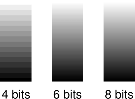
Each color in each channel is made up of so many bits. Most computer images use 8-bits in an unsigned format for `2^8 = 256` different values or shades. Where higher values are usually defined to appear brighter or have a greater intensity. Increasing the number of bits makes the apparent change between different shades of a color smoother. There are also other formats like floats which are clamped to between 0.0 (none) and 1.0 (full intensity) before being displayed.

Images are usually laid out in memory as large continuous blocks. The dimensions used to describe these blocks (think width and height) determines if an image is 1D, 2D (most common and the only type used here), 3D, or something else entirely. The channels can be interleaved (RGBRGBRGBRGB…) or in continuous chunks (RRR…GGG…BBB…). The beginning is usually the top left of the image and successive elements are found in a left-to-right and then top-to-bottom order. Although, some libraries and image storage formats expect the rows in a reversed bottom-to-top order. Accessing a particular pixel’s color channel using an X and Y coordinate is done using a straight forward formula1.
| Format | Example | How to calculate an offset |
|---|---|---|
| Interleaved | RGBRGBRGB | `text{offset} = (y * text{image}_text{width} + x) * text{channel}_text{count} + text{channel}_text{index}` |
| Chunked | RRRGGGBBB | `text{offset} = text{channel}_text{index} * text{image}_text{width} * text{image}_text{height} + y * text{image}_text{width} + x` |
When a camera captures an image, extra processing is almost always done by the hardware2. When done automatically, this processing becomes a characteristic of the camera. Unfortunately, this can be a problem for some image processing algorithms. Since it’s not a problem for the algorithms used in this project, the extra processing won’t be covered here. But, it’s worth investigating if you plan to work on, for example, scientific image processing where you have control over the types of cameras being used.
Color Models and Spaces
There are other ways to represent color than just mixing shades of red, green, and blue (RGB) light. For example, painters mix cyan, magenta, and yellow (CMY) together to form other colors. Another method is to refer to a color by its hue, saturation, and lightness (HSL). These are all examples of color models. Some color models, such as RGB and HSL, allow colors to be converted between one another at a cost of computational precision. In other cases, colors cannot be directly converted, like RGB and CMY, so a much more complicated transform is necessary to match colors that appear similar.
Color spaces describe how a specific color should be perceived. They’re usually defined as a range of colors relative to what can be perceived by humans. Supporting all visible colors doesn’t always make sense. For example, your computer screen cannot display many shades of green that you have no problem seeing (unless you have a vision disability like being color blind). The important take away for color spaces is that if you have an 8-bit RGB value (eg. (255,128,23)) in one color space and the same RGB value in another color space, they don’t necessarily represent the same perceived color.
The industry has standardized around the idea that for any RGB image where a color space is not provided, it’s assumed to use the sRGB color space. Since this project is expected to work with any random camera, this is also the color space assumed for RGB images here. Finding the actual color space of a camera requires a calibration process that is outside the scope of this post.
Basic Image Processing Patterns
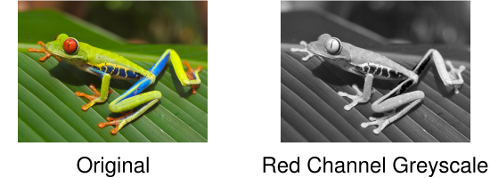
Most of our image processing operations are based on one of two patterns. The first modifies each each pixel independently. Usually in sequential order, for simplicity and cache-efficiency, but order doesn’t really matter. For example, the following copies the red channel value to the green and blue channels to create a type of greyscale image.

constexpr unsigned int RED_CHANNEL_OFFSET = 0;
constexpr unsigned int GREEN_CHANNEL_OFFSET = 1;
constexpr unsigned int BLUE_CHANNEL_OFFSET = 2;
constexpr unsigned int CHANNEL_COUNT = 3;

Image image; //RGB interleaved, unsigned 8-bits per channel.
const unsigned int pixelCount = image.width * image.height;

//Iterate over every pixel.
for(unsigned int x = 0;x < pixelCount;x++)
{
    //Offset to the current pixel.
    const unsigned int index = x * CHANNEL_COUNT;

    //Copy the value in the red channel to both the green and blue channels.
    const unsigned char redValue = image.data[index + RED_CHANNEL_OFFSET];
    image.data[index + GREEN_CHANNEL_OFFSET] = redValue;
    image.data[index + BLUE_CHANNEL_OFFSET] = redValue;
}
The second pattern involves accessing not just a particular pixel, but also the surrounding pixels, to perform an operation known as a convolution. These surrounding pixels are usually accessed in a square shape where each side is some odd number so it fits symmetrically over the center pixel. The center pixel and all surrounding pixels are multiplied by a number defined as part of a kernel and then summed. This summed value then becomes the new value for the center pixel.
You might be wondering: what should be done when the surrounding pixels don’t exist because they are outside the boundary of the image? It completely depends on the operation being performed and how the result is going to be used. Sometimes the edges are not important so the pixels are just skipped. Other times, a clamping behavior is performed so the closest valid pixels are used. There are also algorithms that adapt by changing their behavior such as accessing less pixels and using different kernels.
Here is an example where the edges are ignored and the kernel computes an average to produce a blurred version of the original image.

constexpr unsigned int KERNEL_RADIUS = 2;
constexpr unsigned int KERNEL_DIAMETER = KERNEL_RADIUS * 2 + 1;
constexpr unsigned int KERNEL_SIZE = KERNEL_DIAMETER * KERNEL_DIAMETER;
constexpr unsigned int CHANNEL_COUNT = 3;

Image inputImage; //RGB interleaved, unsigned 8-bits per channel.
Image outputImage; //Same size and format as input image.
const unsigned int rowSpan = inputImage.width * CHANNEL_COUNT;

//Convenience function for getting the pixel of an image at a specific coordinate.
auto GetPixel = [](Image& image,const unsigned int x,const unsigned int y)
{
    assert(x < image.width && y < image.height);

    return &image.data[(y * image.width + x) * CHANNEL_COUNT];
};

//Perform blur convolution on every pixel where the kernel fits completely within the
//image.
for(unsigned int y = KERNEL_RADIUS;y < inputImage.height - KERNEL_RADIUS;y++)
{
    for(unsigned int x = KERNEL_RADIUS;x < inputImage.width - KERNEL_RADIUS;x++)
    {
        //Sum centered and surrounding pixels. Each channel is done individually.
        float sum[CHANNEL_COUNT] = {0.0f};
        for(unsigned int i = 0;i < KERNEL_DIAMETER;i++)
        {
            for(unsigned int j = 0;j < KERNEL_DIAMETER;j++)
            {
                const unsigned char* pixel = GetPixel(inputImage,
                                                      x - KERNEL_RADIUS + j,
                                                      y - KERNEL_RADIUS + i);
                for(unsigned int c = 0;c < CHANNEL_COUNT;c++)
                {
                    sum[c] += pixel[c];
                }
            }
        }

        //Use the sums to compute the average of the centered and surrounding pixels. This
        //is equivalent to a kernel where every entry in the kernel is 1 / KERNEL_SIZE.
        for(unsigned int c = 0;c < CHANNEL_COUNT;c++)
        {
            unsigned char* pixel = GetPixel(outputImage,x,y);
            pixel[c] = std::lrint(sum[c] / static_cast<float>(KERNEL_SIZE));
        }
    }
}
Notice in this example that there are separate input and output images. Because convolutions require the original pixels, modifying the original image in place would produce a completely different and incorrect result.
Greyscale
Many image processing operations expect to work with greyscale images. An earlier example created a greyscale image by copying the red channel to the green and blue channels. When the red, green, and blue channels are equal, the resulting image appears as various shades of grey. There are many different ways to create greyscale images, each with their own aesthetic and technical benefits.
A good choice because it’s easy to implement and makes use of red, green, and blue channels is Y′ (luma) from the YUV color model. Following the BT.601 specification, Y′ can be found using the following formula.
`Y′ = 0.299 * text{Pixel}_R + 0.587 * text{Pixel}_G + 0.114 * text{Pixel}_B`
The code is very similar to the previous greyscale example. Simply iterate over each pixel individually, calculate Y′, and assign the resulting value to the red, green, and blue channels.

constexpr unsigned int RED_CHANNEL_OFFSET = 0;
constexpr unsigned int GREEN_CHANNEL_OFFSET = 1;
constexpr unsigned int BLUE_CHANNEL_OFFSET = 2;
constexpr unsigned int CHANNEL_COUNT = 3;

Image image; //RGB interleaved, unsigned 8-bits per channel.
const unsigned int pixelCount = image.width * image.height;

for(unsigned int x = 0;x < pixelCount;x++)
{
    const unsigned int index = x * CHANNEL_COUNT;

    const unsigned char greyValue =
        0.299f * static_cast<float>(image.data[index + RED_CHANNEL_OFFSET]) +
        0.587f * static_cast<float>(image.data[index + GREEN_CHANNEL_OFFSET]) +
        0.114f * static_cast<float>(image.data[index + BLUE_CHANNEL_OFFSET]);

    image.data[index + RED_CHANNEL_OFFSET] = greyValue;
    image.data[index + GREEN_CHANNEL_OFFSET] = greyValue;
    image.data[index + BLUE_CHANNEL_OFFSET] = greyValue;
}
You might have noticed that a lot of memory is wasted by having all three channels with the same value. This is definitely something to consider when memory is short or you’re trying to increase performance. Keeping images in an RGB format, even when appearing greyscale, tends to make debugging easier because no extra processing is required to display them. Regardless, I’ll make it clear what type of images are being used, whether it’s RGB, greyscale, or something else entirely.
This is just a taste of image processing. If you want to learn more, check out the resources below. Armed with the basics, it’s time to acquire some images to work with. Next up is capturing video frames from a camera.
Resources
If you’re looking to study image processing in more depth, here’s my recommended learning order:
- You’ll probably want a basic understanding of calculus, linear algebra, probability, and set theory first.
- Read The Scientist and Engineer’s Guide to Digital Signal Processing (the digital version is free!). This book does a great job covering the theory which makes it easier to understand how a lot of common algorithms were originally designed. Feel free to skip chapters 26, 28, and 29 because they are outdated.
- Read Digital Image Processing. This book covers a huge range of topics, does a good job breaking problems into steps, and has plenty of examples. It’s very expensive though.
