
Sudoku Solver AR Part 8: Canny Part 3 (Non-Maximum Suppression)
This post is part of a series where I explain how to build an augmented reality Sudoku solver. All of the image processing and computer vision is done from scratch. See the first post for a complete list of topics.
The whole point of the Canny edge detector is to detect edges in an image. Knowing that edges are a rapid change in pixel intensity and armed with the gradient image created using the method in the previous post, locating the edges should be straight forward. Visit each pixel and mark it as an edge if the gradient magnitude is greater than some threshold value. Since the gradient measures the change in intensity and a higher magnitude means a higher rate of change, you could reason that the marked pixels are in fact edges. However, there’s a few problems with this approach. First, marked edges have an arbitrary thickness which might make it harder to determine if it’s part of a straight line. Second, noise and minor textures that were not completely suppressed by the Gaussian filter can create false positives. And third, edges which are not evenly lit (eg. partially covered by a shadow) could be partly excluded by the selected threshold.

These issues are handled using a mixture of Non-Maximum Suppression, Hysterasis Thresholding, and Connectivity Analysis. Since Non-Maximum Suppression and Hysterasis Thresholding are easily performed at the same time, I’m going to cover them together in this post. Connectivity Analysis will be covered next time as the final step in the Canny algorithm.
Non-Maximum Suppression
Non-Maximum Suppression is a line thinning technique. The basic idea isn’t all that different from the naive concept above. The magnitude of the gradient is still used to find pixels that are edges but it isn’t compared to some threshold value. Instead, it’s compared against gradients on either side of the edge, directed by the current gradient’s angle, to make sure they have smaller magnitudes.
The gradient’s angle points in the direction perpendicular to that of the edge. If you’re familiar with normals, that’s exactly what this is. Then this angle already points to one side of the edge. But both sides of the edge are compared, so rotate the angle 180 degrees to find the other side.
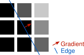
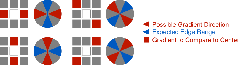
Examine one of these two angles and look at which surrounding pixels it points to. Depending on the angle, it probably won’t point directly at a single pixel. In the example above, instead of pointing directly to the right, it points a little above the right. By the discrete nature of working with images, an approximation must be used to determine a magnitude for comparison on each side of the center gradient. The angle could be snapped to point to the the nearest pixel and respective gradient or an interpolation could be performed between the gradients of the two closest matching pixels. The latter is more accurate but the former is simpler to implement and performs fine for our purpose so that’s the approach used in the code example below.
Hysterasis Thresholding
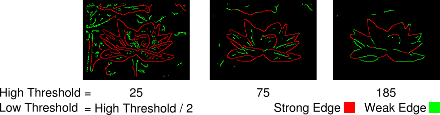
Hysterasis Thresholding is used to suppress edges that were erroneously detected by Non-Maximum Suppression. This could be noise or some pattern that’s too insignificant to be an edge. Perhaps not an obvious solution, but luckily it’s not very complicated. If the magnitude of a gradient is greater than or equal to some high threshold, mark the pixel as a strong edge. If the magnitude of a gradient is greater than or equal to some low threshold, but less than the high threshold, mark the pixel as a weak edge. A strong edge is assumed to be an actual edge where as a weak edge is “maybe” an edge. Weak edges can be promoted to strong edges if they’re directly connected to a strong edge but that’s covered in the next post. The high and low thresholds can be determined experimentally or through various statistical methods outside the scope of this post.
Code
These two concepts are easily implemented together. Start by examining each gradient’s angle to determine which surrounding gradients should be examined. If the current gradient’s magnitude is greater than both the appropriate surrounding gradients’ magnitudes, proceed to hysterasis thresholding. Otherwise, assume the pixel for the current gradient is not an edge. For the hysterasis thresholding step, mark the pixel as a strong edge if it’s greater than or equal to the specified high threshold. If not, mark the pixel as a weak edge if it’s greater than or equal to the specified low threshold. Otherwise, assume the pixel for the current gradient is not an edge. Repeat the process until every gradient is examined.
The following code marks pixels as strong or weak edges by writing to an RGB image initialized to 0. Strong edges set the red channel to 255 and weak edges set the green channel to 255. This could have easily been accomplished with a single channel image where, say, strong edges are set to 1, weak edges set to 2, and non-edges set to 0. The choice of using a full RGB image here is purely for convenience because the results are easier to examine.
const std::vector<float> gradient; //Input gradient with magnitude and angle interleaved
                                   //for each pixel.
const unsigned int width; //Width of image the gradient was created from.
const unsigned int height; //Height of image the gradient was created from.
const unsigned char lowThreshold; //Minimum gradient magnitude to be considered a weak
                                  //edge.
const unsigned char highThreshold; //Minimum gradient magnitude to be considered a strong
                                   //edge.
Image outputImage(width,height); //Output RGB image. A high red channel indicates a strong
                                 //edge, a high green channel indicates a weak edge, and
                                 //the blue channel is set to 0.

assert(gradient.size() == width * height * 2);
assert(lowThreshold < highThreshold);

//Perform Non-Maximum Suppression and Hysterasis Thresholding.
for(unsigned int y = 1;y < height - 1;y++)
{
    for(unsigned int x = 1;x < width - 1;x++)
    {
        const unsigned int inputIndex = (y * width + x) * 2;
        const unsigned int outputIndex = (y * width + x) * 3;

        const float magnitude = gradient[inputIndex + 0];

        //Discretize angle into one of four fixed steps to indicate which direction the
        //edge is running along: horizontal, vertical, left-to-right diagonal, or
        //right-to-left diagonal. The edge direction is 90 degrees from the gradient
        //angle.
        float angle = gradient[inputIndex + 1];

        //The input angle is in the range of [-pi,pi] but negative angles represent the
        //same edge direction as angles 180 degrees apart.
        angle = angle >= 0.0f ? angle : angle + M_PI;

        //Scale from [0,pi] to [0,4] and round to an integer representing a direction.
        //Each direction is made up of 45 degree blocks. The rounding and modulus handle
        //the situation where the first and final 45/2 degrees are both part of the same
        //direction.
        angle = angle * 4.0f / M_PI;
        const unsigned char direction = lroundf(angle) % 4;

        //Only mark pixels as edges when the gradients of the pixels immediately on either
        //side of the edge have smaller magnitudes. This keeps the edges thin.
        bool suppress = false;
        if(direction == 0) //Vertical edge.
            suppress = magnitude < gradient[inputIndex - 2] ||
                       magnitude < gradient[inputIndex + 2];
        else if(direction == 1) //Right-to-left diagonal edge.
            suppress = magnitude < gradient[inputIndex - width * 2 - 2] ||
                       magnitude < gradient[inputIndex + width * 2 + 2];
        else if(direction == 2) //Horizontal edge.
            suppress = magnitude < gradient[inputIndex - width * 2] ||
                       magnitude < gradient[inputIndex + width * 2];
        else if(direction == 3) //Left-to-right diagonal edge.
            suppress = magnitude < gradient[inputIndex - width * 2 + 2] ||
                       magnitude < gradient[inputIndex + width * 2 - 2];

        if(suppress || magnitude < lowThreshold)
        {
            outputImage.data[outputIndex + 0] = 0;
            outputImage.data[outputIndex + 1] = 0;
            outputImage.data[outputIndex + 2] = 0;
        }
        else
        {
            //Use thresholding to indicate strong and weak edges. Strong edges are assumed
            //to be valid edges. Connectivity analysis is needed to check if a weak edge
            //is connected to a strong edge. This means that the weak edge is also a valid
            //edge.
            const unsigned char strong = magnitude >= highThreshold ? 255 : 0;
            const unsigned char weak = magnitude < highThreshold ? 255 : 0;
            outputImage.data[outputIndex + 0] = strong;
            outputImage.data[outputIndex + 1] = weak;
            outputImage.data[outputIndex + 2] = 0;
        }
    }
}
We’re almost done implementing the Canny algorithm. Next week will be the final step where Connectivity Analysis is used to find weak edges that should be be promoted to strong edges. There will also be a quick review and some final thoughts on using the algorithm.